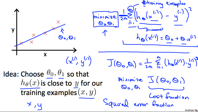
Cost Function

Using the housing price example again, we remember that our hypothesis function will predict the price of the house (y) based on the size in squared feet (x). Therefore our hypothesis, a linear regression equation in this case, is:

$h_θ(x) = θ_0 + θ_1x$

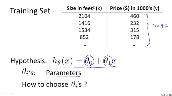
$θ_0, θ_1$ are parameters that will determine how our hypothesis look like.

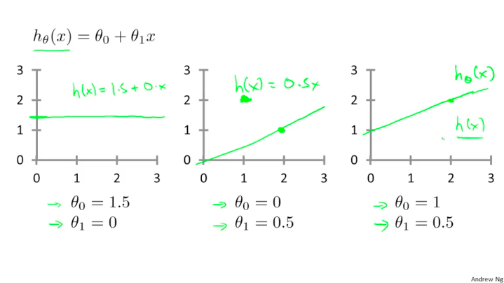
In the picture below, you see that different $θ_0, θ_1$ values produce a different hypothesis. When $θ_0=1.5, θ_1=0$, we get a horizontal line that crosses the (0,1.5) point. When $θ_0=0, θ_1=0.5$ we get a straight line that passes through (0,0) and (2,1) with a gradient of 0.5. When $θ_0=1, θ_1=0.5$, we get a straight line that passes through (0,1) and (2,2) with a gradient of 0.5.

Quiz

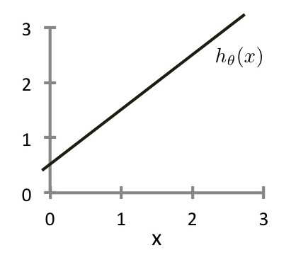
Consider the plot below of $hθ(x) = θ_0 + θ_1x$. What is $θ_0$ and $θ_1$?

• ( ) $θ_0=0, θ_1=1$
• (x) $θ_0=0.5, θ_1=1$
• ( ) $θ_0=1, θ_1=0.5$
• ( ) $θ_0=1, θ_1=1$

We can measure the accuracy of our hypothesis function by using a cost function. This takes an average difference (actually a fancier version of an average) of all the results of the hypothesis with inputs from x's and the actual output y's.

$J(θ_0,θ_1) = \frac{1}{2m} \sum_{i=1}^m \left(\hat{y}_i − y_i\right)^2 = \frac{1}{2m} \sum_{i=1}^m \left( h_θ (x_i) − y_i \right)^2$

To break it apart, it is $\frac 12 \bar x$ where $\bar x$ is the mean of the squares of $h_θ(x_i) − y_i$ , or the difference between the predicted value and the actual value.

This function is otherwise called the "Squared error function", or "Mean squared error". The mean is halved $\left( frac 12 \rigth)$ as a convenience for the computation of the gradient descent, as the derivative term of the square function will cancel out the $frac 12$ term. The following image summarizes what the cost function does: